I. Assumptions, rationality, risk-aversion, and types of games
A decision has three features:
- Actions an agent can choose,
- Possible consequences of these actions (outcomes), and
- preference relations between these outcomes, e.g. x_1 \succ x_2 for strong preference and x_1 \succeq x_2 for weak preference.
A payoff function quantifies the utility from an outcome (so if v(x_1) \geq v(x_2), then x_1 has \geq payoff function value, and x_1 \succ x_2)
By assumptions of transitivity (if v(x_1) > v(x_2) and v(x_2) > v(x_3), then v(x_1) > v(x_3) – see Condorcet paradox) and completeness (for any outcome x_n in x, either x_1 \succ x_2, x_2 \succeq x_1, or both)
\rightarrow Proposition 1.1: If a set of outcomes x is finite, then any rational preference relation over x can be represented by a payoff function.
\rightarrow Definition 1.2: An agent faced with a decision problem is rational if the agent chooses a^* such that v(x(a^*)) \geq v(x(a)) for all possible choices of a; or, in other words, if this agent maximizes the payoff function.
Games can be displayed in such forms as functions, matrices, and decision trees:
1. Cournot Duopoly: Games as functions
The Cournot Duopoly is defined as follows, in normal form:
- N = \{1,2\} (2 players)
- S_i = [0, \infty) (possible strategies give 0 to \infty)
- v_i(s_i, s_j) = (100 - s_i - s_j) \cdot s_i - s_i^2 (payoff function given strategies s_i and s_j)
To maximize v_i, we can first rewrite it as 100 s_i - 2s_i^2 - s_i\cdot s_j. Then, taking the derivative and setting it equal to 0: \frac{\partial v_i}{\partial s_i} = 100 - 4s_i - s_j = 0
Rearranging to get s_i, we have s_i = \frac{100 - s_j}{4}. If we plug in the minimum value for s_j, we can get an upper bound on the value of s_i: \frac{100 - 0}{4} = 25 Since s_i is bounded above at 25, we can repeat this from the angle of s_j as follows: \frac{100 - 25}{4} = 18.75 …giving us a lower bound on the value of s_j. We can make a simple program to do this in Python, stopping when we either iterate more than 1000 times or we are within \frac{1}{10000} of the value we had at the previous iteration:
x = 0; prev_x = -float('inf')
iters = 0
while abs(x - prev_x) > 1e-4 and iters < 1000:
    prev_x = x
    x = (100 - x)/4
    iters += 1
print(round(x,2))
=> 20.0Alternatively, this problem happens to be solvable using the second derivative (as the interval does indeed converge to a single value) as follows: \frac{\partial v_i}{\partial s_i^2} = - 4
Since -4 < 0, we know that v_i is concave down. Therefore, there must be one point which maximizes the function, which we can solve for using a system of equations, along with the use of symmetry and first-derivative optimization: \begin{aligned} 100 - 4s_i -s_j &= 0 \\ 100 - 4s_i &= s_j \\ 100 - 4(100 - 4s_j) &= s_j \\ 100 - 400 + 16s_j &= s_j \\ -300 &= -15s_j\\ s_i = s_j &= 20 \end{aligned}
Note that taking the second derivative and solving a system of equations is not guaranteed to yield the correct answer, as it does not work for ranges of answers. It is, however, a useful tool to check one’s work.
2. R&D Problem: Games as decision trees
Example decision tree game:
- N = \{1\} (this is more of a decision than a game)
- S_i = \{\text{go}, \text{don't go}\}
- v_i depends on successes and failures, and is defined using the following tree:
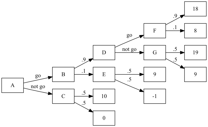
We use expected values and backwards induction to find the optimal choice of [A, G]: \begin{aligned} F &= 18(.9) + 8(.1) = 17 \\ G &= 19(.5) + 9(.5) = 14 \\ D &= \max(F,G) = \max(17,14) = 17 \quad \text{by rationality} \\ E &= 9(.5) + -1(.5) = 4 \\ B &= D(.9) + E(.1) = 17(.9) + 4(.1) = 15.7 \\ C &= 10(.5) = 5 \\ \text{(expected payoff)}\quad A &= 15.7, \quad \text{found by \textit{going}} \end{aligned}
Note that if going increased P(\text{success}) to .6 instead of .9, it would probably be best not to go.
Risk-neutral implies that v(x) = x; this may not be the case in real life, where a downside generally hurts more than an upside helps.
To show that most people are risk-averse rather than risk-neutral, consider the following scenario: A person can accept $1000, or they can flip some number of coins given by sequence c with the following rewards: \text{reward}(c) = \begin{cases} \$1 & c = [t] \\ \$2 & c = [h;t] \\ \$4 & c = [h;h;t] \\ \vdots & \vdots \\ \$\infty & c = [\underbrace{h; \dots}_{\infty \text{ times}};t] \end{cases}
The expected value of the above reward is, where h_c is the number of h flips in sequence c: \sum_{h_c=0}^\infty 2^{h_c} \left(\frac{1}{2}\right)^{h_c} = \$\infty
However, few people would take the coin flips: people are risk-averse.
3. The Prisoner’s Dilemma: Games as matrices
The Prisoner’s Dilemma problem is defined as follows:
- N = \{1,2\}
- S_i = \{C := \text{confess}, S := \text{stay silent}\}
- v_i(s_i, s_j) is symmetric with the following payoffs:
- v_i(C,C) = -4
- v_i(C,S) = -1
- v_i(S,C) = -5
- v_i(S,S) = -2
This can be written as a matrix like so: \begin{array}{r||c|c} P1 \backslash P2& C & S \\ \hline \hline C & (-4,-4) & (-1,-5) \\ \hline S & (-5,-1) & (-2,-2) \end{array}
What should a player do in this scenario? Strategies will tell us.
II. Strategies for pure games: IESDS, Rationalizability, and Nash Equilibrium
A static game with complete information is a game, like above, where every player chooses an action simultaenously and independently, and all players know all possible actions of all players, all possible outcomes, the outcomes that result from the given actions, and the payoffs of all players. Pure strategies are deterministic plans of actions a player takes in every “situation of the game”.
We say that strategy A is strictly dominated by strategy B if the payoff of strategy B beats the payoff of strategy A in all situations. For example, in the Prisoner’s Dilemma example above, since -4 > -5 and -1 > -2, P2’s action C strictly dominates S. The same is true for P1 by symmetry, so the strictly dominant strategy that remains is [C,C].
\rightarrow By Claim 4.1, a player that is rational will never play a strictly dominated strategy.
Thus, the only rational choice for each player is to choose C.
Strategy 1: IESDS
The self-explaining IESDS (Iterated Elimination of Strictly Dominated Strategies) method eliminates strictly dominated strategies.
Example (A): 3\times 3 matrix
Consider the following game, given in normal form with payoff matrix below:
- N = \{1,2\}
- S_1 = \{U,M,D\}
- S_2 = \{L,C,R\}
\begin{array}{r||c|c|c} P1 \backslash P2& L & C & R \\ \hline \hline U & (4,3) & (5,1) & (6,2) \\ \hline M & (2,1) & (8,4) & (3,6) \\ \hline D & (3,0) & (9,6) & (2,8) \end{array}
We use IESDS as follows:
- For P2: 2 > 1, 6 > 4, and 8 > 6, so C is strictly dominated by R
- For P1: 4 > 2 and 4 > 3, and 6 > 3 and 6 > 2; therefore, M and D are strictly dominated by U
- For P2: 3 > 2, so R is strictly dominated by L.
Therefore, [U,L] is the solution by IESDS.
Example (B): Cournot Duopoly
See above: I \rightarrow 1. Cournot Duopoly. The convergence method is really an example of IESDS.
Example (C): Second-price auction
Strong dominance is not the only means of selecting a strategy. Consider a second-price auction, wherein players bid and the player with the highest bid only pays the amount of the second-highest bid. A small example, with only 2 players, could be defined as follows:
- Player P1, who values the item at price v_1, bids b_1
- Player P2, who values the item at price v_2, bids b_2
- The profit for player i is v_i - b_{i+1\text{ mod } 2} if player i wins, and 0 otherwise.
We then have the following cases for P1: \text{profit} = \begin{cases} \begin{cases} 0 & v_1 = b_2 \\ - & v_1 < b_2 \\ + & v_1 > b_2 \end{cases} & b_1 > b_2 \\ 0 & b_1 < b_2 \end{cases}
So, P1 only loses when v_1 < b_2 < b_1, which cannot happen if b1 = v1. Therefore, b_1 = v_1 is weakly dominant: that is, there is at least one scenario in which it is equal to other strategies, but there is also at least one scenario in which it dominates other strategies. Since the strategy is weakly dominant, it is also a best response.
Strategy 2: Best responses and rationalizability
A best response is, given all opponent strategies, the best strategy a player can play. In other words: BR_i = s_i^* \iff v_i (s_i^*, s_{-i}) \geq v_i(s_i, s_{-i}) \quad \forall s_i \in S_i.
If we look at the 3\times 3 matrix example from the previous part, we see that:
- BR_1(L) = U, BR_1(C) = D, and BR_1(R) = U
- Therefore, it is never in the best interest of player P1 to play M
- BR_2(U) = L, BR_2(M) = R, and BR_2(D) = R
- Therefore, it is never in the best interest of player P2 to play C
Repeating with those choices taken out gives:
- BR_1(L) = U and BR_1(R) = U
- Therefore, it is never in the best interest of player P1 to play D
- BR_2(U) = L and BR_2(D) = R
So, since BR_1(L) = U and BR_2(U) = L, we know that [U,L] is the rationalizable equilibrium.
Proposition 4.3: A strictly dominated strategy cannot be a best response, beacuse if v_i(s_i^*, s_{-i}) < v_i(s_i, s_{-i}) for some s_i, then v_i(s_i^*, s_{-i}) \not\geq v_i(s_i, s_{-i}) for that s_i.
Example: IESDS equilibria vs. rationalizable equilibria
However, the set of rationalizable equilibria is a subset of IESDS equilibria. Consider the following game:
\begin{array}{r||c|c} P1 \backslash P2& L & R \\ \hline \hline U & (3,0) & (0,0) \\ \hline M & (0,0) & (3,0) \\ \hline D & (1,0) & (1,0) \end{array}
According to IESDS, there are no strongly dominated strategies. Therefore, all 6 of the possible strategies survive IESDS: \text{IESDS} \implies \{[L,U], [R,U], [L,M], [R,M], [L,D], [R,D]\}
We can, however, pare down the strategies using best responses as follows:
- BR_1(L) = U and BR_1(R) = M, so P1 will never play D
- BR_2(U) = BR_2(M) = BR_2(D) = \{L, R\}. We can’t really say anything about P2.
With this alone we reduce the size of our outcome set by \frac{1}{3}: \text{BR} \implies \{[L, U], [R, U], [L,M], [R,M]\}
Strategy 3: Nash equilibria
A Nash equilibrium of [A, B] between players i and j holds when BR_i(A) = B and BR_j(B) = A, or more formally: s_i^* \in BR_i (s_{-i}^*) \quad \forall i.
In the above example, BR_1(L) = U, BR_2(U) = L, BR_1(R) = M, and BR_2(M) = R, so the set of Nash equilibria is \{[L,U], [R,M]\}.
Proposition 5.1: If a strategy profile is a strictly dominant strategy equilibrium, a unique IESDS survivor, or a unique rationalizable strategy profile, it is a Nash equilibrium.
Unfortunately, rational actors’ collective selfishness ends up detracting from the greater good. This is called the Tragedy of the Commons.
For example, if there are K units of clean air, each firm i uses k_i units, and payoffs v_i(k_i, k_{-i}) are v_i(k_i, k_{-i}) = \ln(k_i) + \ln\left(K - \sum_{j} k_j\right),
then we have the following: BR_i(k_i) = \text{argmax}_{k_i} \left[\ln\left(K - \sum_{j} k_j\right)\right] \begin{aligned} \frac{\partial v_i(k_i, k_{-i})}{\partial k_i} &= \frac{1}{k_i} + \frac{1}{K - \sum_{j} k_j}(-1) = 0 \\ \frac{1}{k_i} &= \frac{1}{K - \sum_{j} k_j} \\ k_i &= K - \sum_{j} k_j \\ &= K - \left[\left(\sum_{j\neq i} k_j\right) + k_i\right] \\ 2k_i &= K - \sum_{j\neq i} k_j \\ k_i &= \frac{1}{2} \left(\sum_{j\neq i} k_j\right) \end{aligned}
If there are 2 firms, then k_1 = k_2 = \frac{1}{3} K at the Nash equilibrium.
A government, on the other hand, would maximize total welfare: w := \ln(k_1) + \ln(K - k_1 - k_2) + \ln(k_2) + \ln(K - k_2 - k_1) \frac{\partial w}{\partial k_1} = \frac{1}{k_1} - \frac{2}{K - k_1 - k_2}
By symmetry, setting \frac{\partial w}{\partial k_1} = 0 reveals k_1 = k_2 = \frac{1}{4}K at the government optimum. Thus, the Nash equilibrium of a game is not necessarily the best for total welfare.
III. Mixed strategies
Some games have no pure strategy Nash equilibrium. In Rock-Paper-Scissors, for instance:
- BR(\text{Rock}) = \text{Paper}$
- BR(\text{Paper}) = \text{Scissors}$
- BR(\text{Scissors}) = \text{Rock}$
(Note that the above relationships and the symmetry of the above game imply that the game is not transitive.)
If S_i = \{s_1, \dots, s_n\} is the pure strategy set for player i, we define mixed strategies to be of the form “s_{ik} played with probability \sigma_i(s_{ik})”, or in the case of Rock-Paper-Scissors: \sigma_1(R) = \frac{1}{3} \quad \sigma_1(P) = \frac{1}{3} \quad \sigma_1(S) = \frac{1}{3}
Note that \sum_k s_{ik} = 1. In pure strategies, \sigma_i(s_i) = 1 for any s.
Definitions regarding mixed strategies
\rightarrow Definition 6.3: Over interval S_i, a mixed strategy for player i is a CDF (cumulative distribution function) F_i : S_i \rightarrow [0,1] where a player plays s_i \leq x with probability \Pr(s_i\leq x) = F_i(x). If F_i(\cdot) is differentiable with density f_i(\cdot), then we say that s_i\in S_i is in the support of F_i(\cdot) if f_i(s_i) > 0; or in other words, s_i’s rationality as a strategy is vouched for by F_i if f_i(s_i) > 0.
\rightarrow Definition 6.4: A belief of player i is a probability distribution \pi_i\in \Delta S_{-i} over the strategies of his opponents. We denote the probability player i assigns to his opponents playing s_{-i} \in S_{-i} as \pi_i(s_{-i}).
\rightarrow Definition 6.5: The expected payoff of player i when he chooses pure strategy s_i\in S_i and all other players play mixed strategies \sigma_{-i}\in \Delta S_{-i} is as follows: v_i(s_i, \sigma_{-i}) = \sum_{s_{-i}\in S_{-i}} \sigma_{-i} (s_{-i}) v_i (s_i, s_{-i}).
Similarly, the expected payoff of player i when he chooses mixed strategy \sigma_i\in \Delta S_i and all other players play mixed strategies \sigma_{-i}\in \Delta S_{-i} is as follows: \begin{aligned} v_i(\sigma_i, \sigma_{-i}) &= \sum_{s_{i}\in S_{i}} \sigma_{i} (s_{i}) v_i (s_i, \sigma_{-i}) \\ &= \sum_{s_i\in S_i} \left(\sum_{s_{-i}\in S_{-i}} \sigma_{-i} (s_{-i}) v_i (s_i, s_{-i})\right) \end{aligned}
Example (A): Rock-Paper-Scissors
For example, in Rock-Paper-Scissors, if player 2 plays the following \sigma_2… \sigma_2(R) = \sigma_2(P) = \frac{1}{2}, \sigma_2(S) = 0
…then we get the following payoffs for player 1:
- v_1(R, \sigma_2) = \frac{1}{2} (-1) + \frac{1}{2} (0) = -\frac{1}{2}
- v_1(P, \sigma_2) = \frac{1}{2} (0) + \frac{1}{2} (1) = \frac{1}{2}
- v_1(S, \sigma_2) = \frac{1}{2} (1) + \frac{1}{2} (-1) = 0
Thus, the best response is \{P\}. This makes intuitive sense given that no matter what, P can never be beaten by player 2 because they never play S.
Example (B): Nickel-Dime game
We define the Nickel-Dime game as follows:
\begin{array}{r||c|c} P1 \backslash P2& N & D \\ \hline \hline N & (5,-5) & (-5,10) \\ \hline D & (-10,5) & (10,-10) \end{array}
In calculating the Nash equilibrium for the above game, assume that P2 plays \sigma_2, and that p = \Pr(\text{Nickel}) and that 1-p = \Pr(\text{dime}).
We calculate the Nash equilibria using best-responses as follows:
- BR_1(N, \sigma_2) = 5p + -10(1-p) = 15p-10
- BR_1(D,\sigma_2) = -5p + 10(1-p) = -15p+10
The best choice for P1 depends on p, and can be calculated as follows: \begin{aligned} 15p - 10 &> -15p + 10 \\ -20 &> -30p \\ 2 &< 3p \\ \frac{2}{3} &< p \end{aligned}
Thus, if p > \frac{2}{3}, then BR_1 is N.
And assuming the opposite for player P1:
- BR_2(N,\sigma_1) = -5q + 10(1-q) = -15q+10
- BR_2(D, \sigma_1) = 5q + -10(1-q) = 15q-10
And with similar calculations: \begin{aligned} -15p - 10 &> 15p + 10 \\ -30q &> -20 \\ 3q &< 2 \\ q &< \frac{2}{3} \end{aligned}
So if q < \frac{2}{3}, then BR_2 is N as well.
It turns out that if p = q = \frac{2}{3}, then the players are indifferent about their choice between N and D.
For either player: P1: BR_1((p, 1-p)) = \begin{cases} N & p > \frac{2}{3} \\ D & p < \frac{2}{3} \\ \{N,D\} & p = \frac{2}{3} \end{cases} P2: BR_2((q, 1-q)) = \begin{cases} N & q < \frac{2}{3} \\ D & q > \frac{2}{3} \\ \{N,D\} & q = \frac{2}{3} \end{cases}
In the last of the three cases for each of these, any mixed combination of N or D has equal expectation.
Note that the Nash equilibrium here is (in the form (N,D)): \left[\left(\frac{2}{3}, \frac{1}{3}\right), \left(\frac{1}{3}, \frac{2}{3}\right)\right]
By Proposition 6.1, if \sigma^* = (\sigma_1^*, \sigma_2^*, \dots, \sigma_n^*) is a Nash equilibrium, and player P1 has pure strategies s_i and s_i' as well as mixed strategy \sigma_i^* which is a combination of s_i and s_i', then v_i is as follows: v_i(s_i, \sigma_{-i}^*) = v_i(s_i^*, \sigma_{-i}^*) = v_i(\sigma_i, \sigma_{-i}).
If this were not the case – say, v_i(s_i, \sigma_{-i}^*) < v_i(s_i', \sigma_{-i}^*) – then it would never be better to play s_i' over s_i. If a player is randomizing between two strategies, the player must be indifferent between them. The reason for playing a mixed strategy is so that another player cannot intuit the original player’s strategy.
Example (C): 2\times 2 matrix
Consider the following example: \begin{array}{r||c|c} P1 \backslash P2& C & R \\ \hline \hline M & (0,0) & (3,5) \\ \hline D & (4,4) & (0,3) \end{array}
By pure strategy:
- BR_1(C) = D, BR_1(R) = M
- BR_2(M) = R, BR_2(D) = C
So [C,D] and [M,R] are pure equilibria.
For a mixed strategy:
-
v_1(M, \sigma_2^*) = \sigma_2^*(C) v_1(M,C) + \sigma_2^*(R) v_1(M,R)
-
v_1(D, \sigma_2^*) = \sigma_2^*(C) v_1(D,C) + \sigma_2^*(R) v_1(D,R)
-
v_1(M,\sigma_2^*) = 3\sigma_2^*(R) = 2(1-\sigma_2^*(C)) = 3 - 3\sigma_2^*(C)
-
v_1(M,\sigma_2^*) = 4\sigma_2^*
So: \begin{aligned} 3 - 3\sigma_2^*(C) &> 4\sigma_2^* \\ 3 &> 7\sigma_2^* \\ \frac{3}{7} &> \sigma_2^* \end{aligned}
Thus, \sigma_2^* = (\Pr(C), \Pr(R)) = \left(\frac{3}{7}, \frac{4}{7}\right).